Starscapes on Algebraic Surfaces
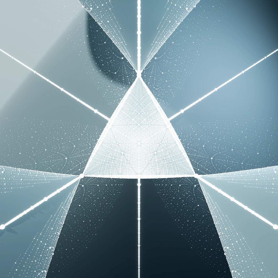
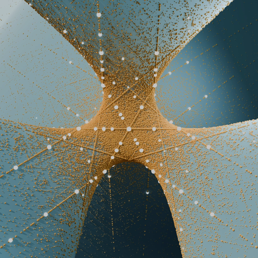
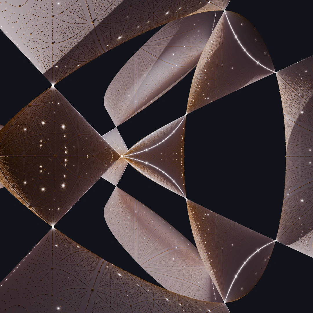
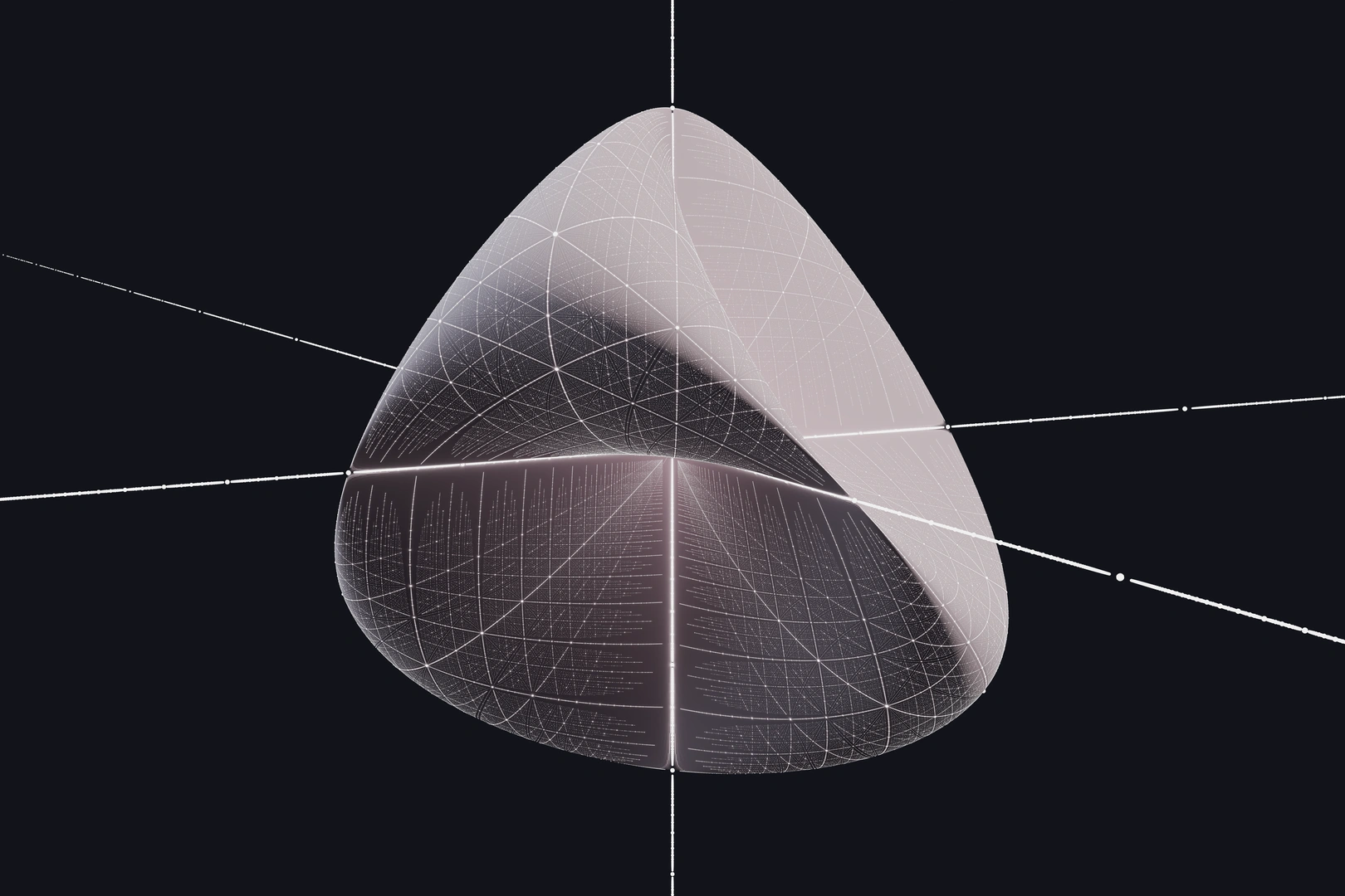
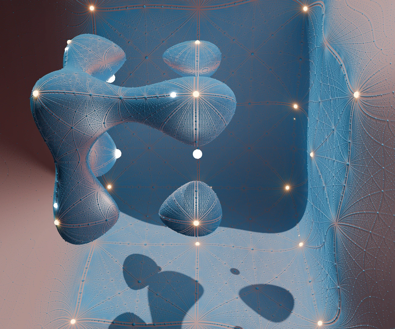
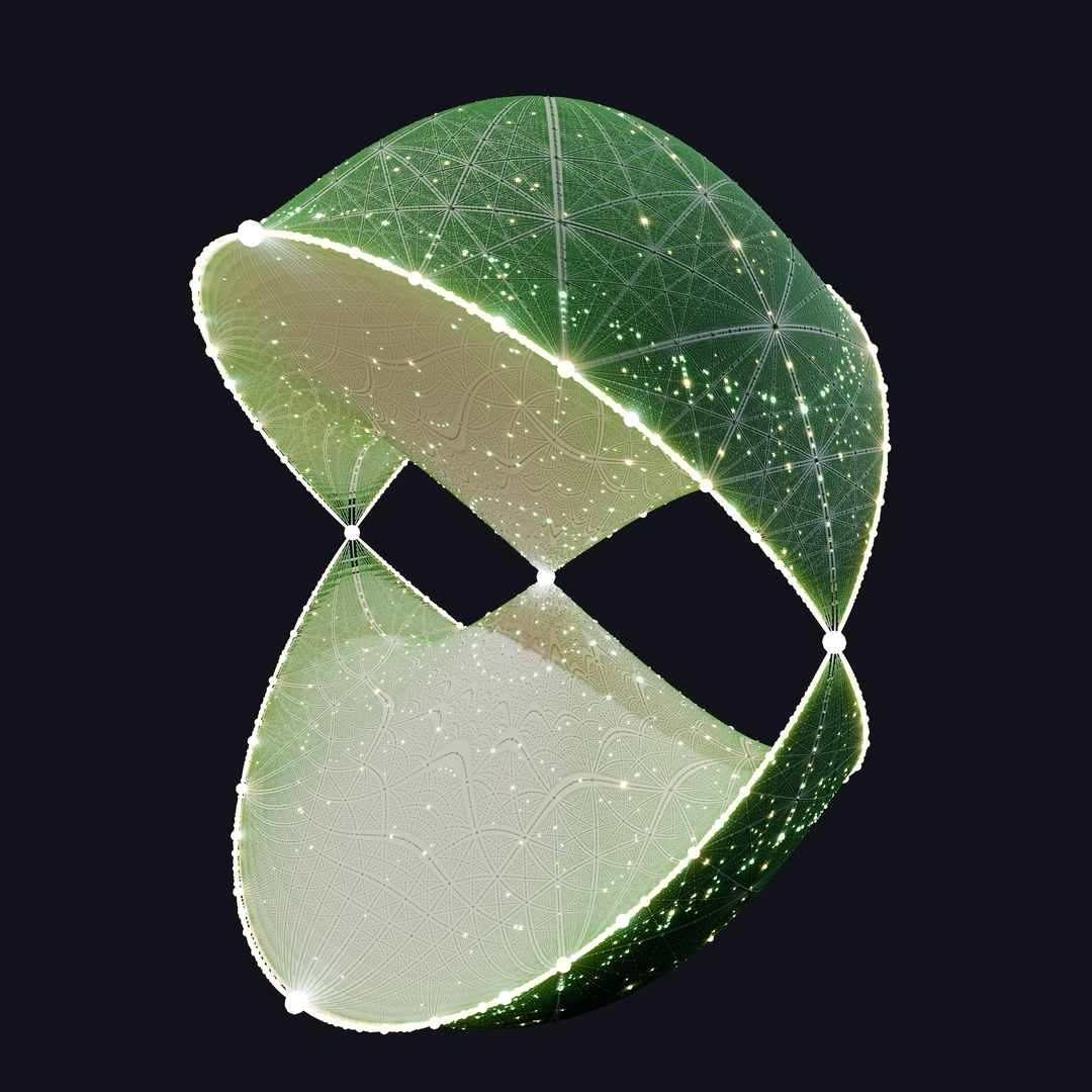
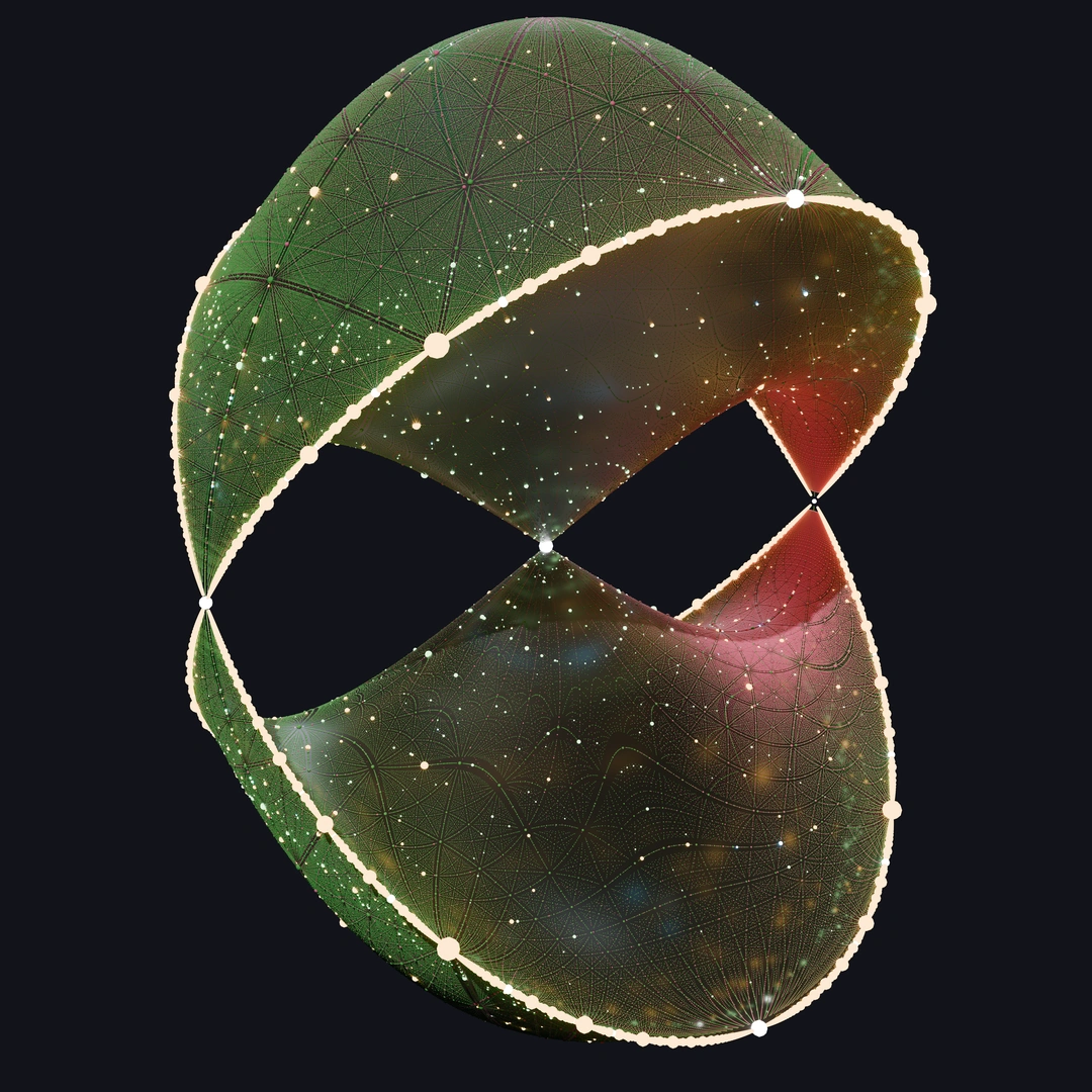
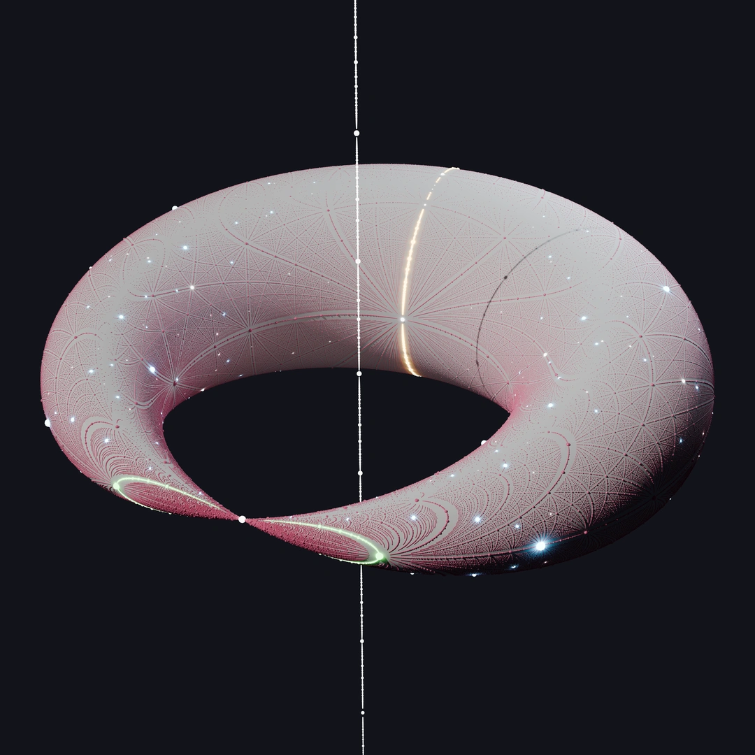
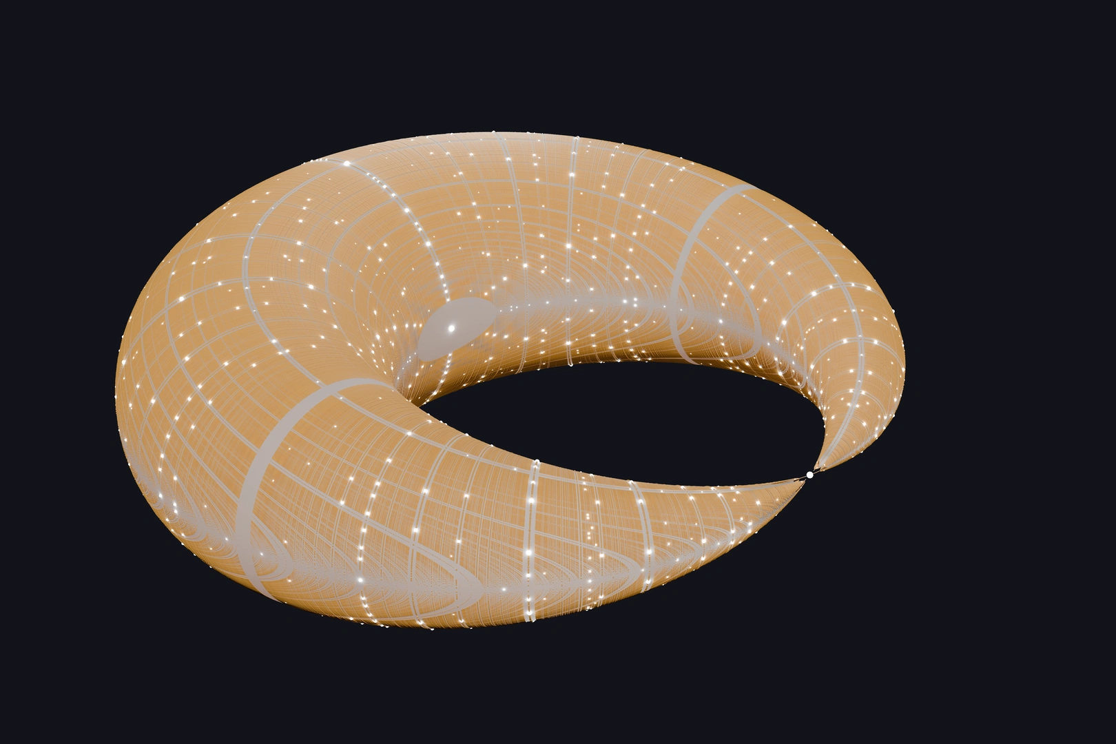
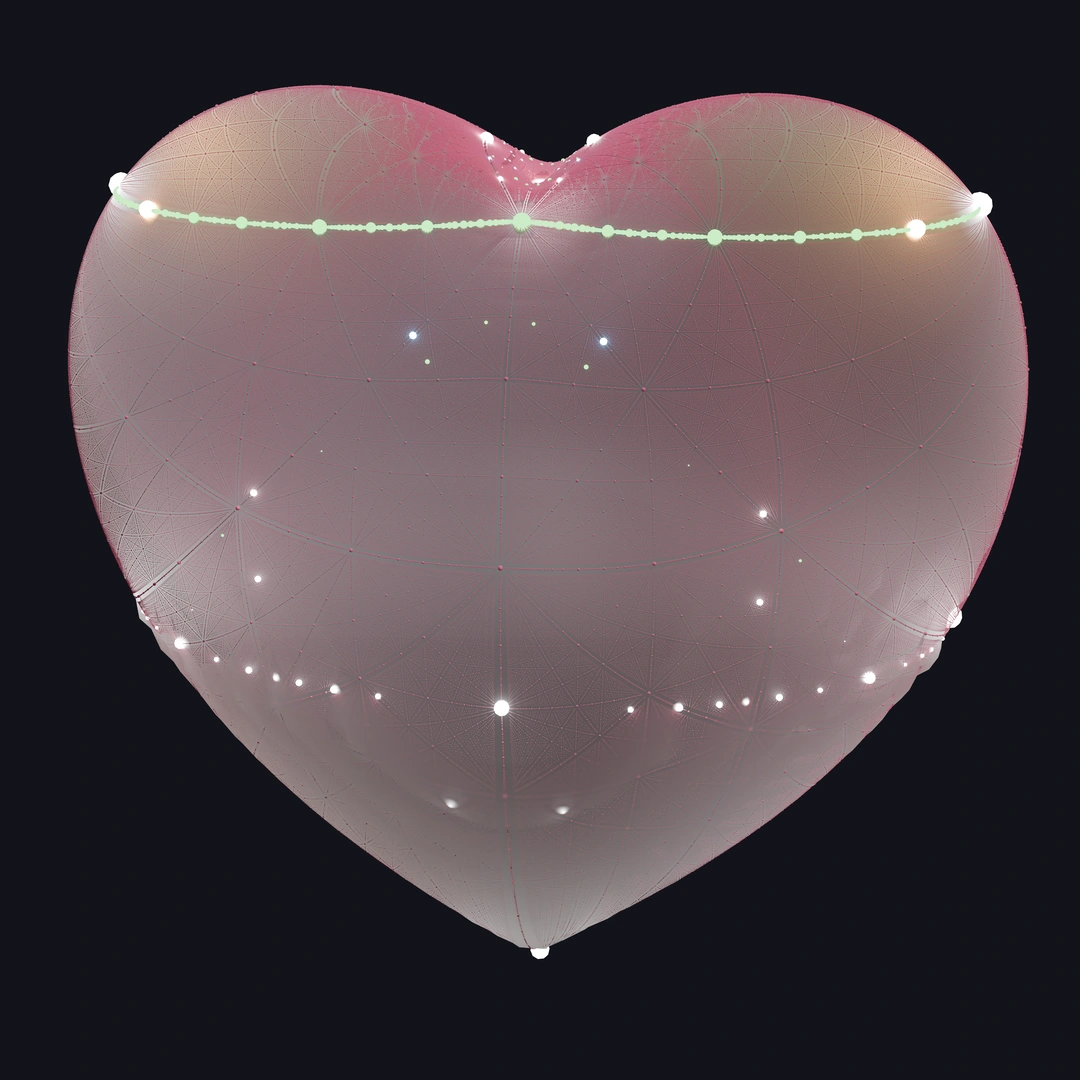
Check out the Isolated Nodal Quintic, Croissant Sextic, and Taubin Sextic (0,0,1) in the gallery below.
This project developed alongside other mathematical research joint with Jesse Wolfson and Alexander Sutherland. These led, among other things, to several papers: (Gómez-Gonzáles, Sutherland, and Wolfson 2024; Gómez-Gonzáles and Wolfson 2025; Gómez-Gonzáles 2026).
Special Points
A crucial idea throughout all three is the question of exhibiting dense supplies of special classes of points on certain algebraic varieties (i.e., geometric spaces defined by systems of polynomial equations). Being fans of resolvent degree, we are particularly interested in the solvable points and level \(\ell\) points of a variety. These are points whose coordinates can be expressed in radicals or, more generally, using algebraic functions of at most \(\ell\) variables.
In the last two of these papers, we build on work of Sutherland and Heberle to establish techniques for obtaining these special points—indeed, often many of them! The fundamental idea dates back at least to an algorithm of James Joseph Sylvester (circa 1886), which uses lines and other linear subspaces to reduce the a priori hard problem of finding points on a variety into easier problems. In the gallery below, we pursue this theme through various tricks involving singular loci and lines contained in the surfaces, allowing us to identify whole swathes of points whose arithmetic complexity is much lower than a random geometric sampling would yield.
Be particularly attentive to how the points below seem to “fill in” the surfaces on which they sit. This visualizes the notion of density crucial to our papers, showing that, despite belonging to restricted arithmetic strata, these special points often still blanket the variety.
To each point we find, we can associate a Galois group—the algebraic object describing the complexity of the field extension required to define the point. While a generic line intersecting a degree \(d\) surface yields a point saddled with the full symmetric group \(S_d\), our geometric constructions unearth dense sets of points governed by more accessible groups.1 Indeed, the white points below (marked by \(C_1\) in the legend) are good, old-fashioned rational numbers!
Special Points Applet
Cayley Cubic, projecting from the origin \[x\ y\ z + (1 - x - y - z)(x\ y + x\ z + y\ z) = 0\]
Clebsch Cubic, scanning between 36 skew pairs \[1 + x^3 + y^3 + z^3 - (1 + x + y + z)^3 = 0\]
Fermat Quartic (transformed from its usual form), scanning between 12 skew pairs \[x^4 + y^4 - z^4 - 1 = 0\]
Isolated Nodal Quartic, projecting from the origin \[x^4 + y^4 + z^4 - x\ y\ z - x^2 - y^2 - z^2 = 0\]
Kummer Quartic, projecting from \((1,1,1)\) and \((2,2,4)\) \[(x^4 + y^4 + z^4) - 5 (x^2 y^2 + y^2 z^2 + z^2 x^2) + 56\ x\ y\ z - 20 (x^2 + y^2 + z^2) + 16 = 0\]
Steiner Quartic, projecting from the origin \[x^2 y^2 + y^2 z^2 + z^2 x^2 - x\ y\ z = 0\]
Isolated Nodal Quintic, projecting from the origin \[(x^5 + y^5 + z^5) - (x^4 + y^4 + z^4) - 2(x^3 + y^3 + z^3) + 2(x^2 + y^2 + z^2) = 0\]
Crixxi Sextic, projecting from the origin and \((0,1,0)\) \[(y^2 + z^2 - 1)^2 + (x^2 + y^2 - 1)^3 = 0\]
Croissant Sextic, projecting from \((2,0,0)\) \[(x^2 + y^2)(2x^2 + 2y^2 + 2z^2 + 7)^2 - (8x^2 + 8y^2 - x)^2 = 0\]
Taubin Sextic (Heart), projecting from \((0,0,\pm 1)\) \[(x^2 + \tfrac{9}{4}y^2 + z^2 - 1)^3 - x^2 z^3 - \tfrac{9}{80} y^2 z^3 = 0\]
Nodal Sextic (Two-Sheeted), projecting from the origin \[(x^6 + y^6 + z^6) - 10(x^4 + y^4 + z^4) + (x^2 + y^2 + z^2) = 0\]
Quintuple-Point Sextic, projecting from the origin \[(x^6 + y^6 + z^6) - (x^5 + y^5 + z^5) = 0\]
Stratified Nodal Septic, projecting from the origin \[(x\ y\ z + x - y)\ (x^2 + y^2 + z^2)^2 + (x^2 + y^2 + z^2)^3 + x\ z\ (x^2 + y^2 + z^2) + y\ z^2 + x^2 + y^2 - z^2 = 0\]
Creased Nodal Septic, projecting from the origin \[x\ y\ z (x^2 + y^2 + z^2)^2 + (x + y\ z)(x^2 + y^2 + z^2) + x^2 + y^2 - z^2 = 0\]
Symmetric Nodal Octic (Octahedral), projecting from the origin \[(x^2 + y^2 + z^2)\ \left((x^6 + y^6 + z^6) - 10(x^3 y^3 + y^3 z^3 + z^3 x^3) + 15(x^2 y^2 z^2) \right) + 3(x^4 + y^4 + z^4) - (x^2 + y^2 - z^2) = 0\]
Stratified Nodal Octic, projecting from the origin \[(x\ y + x)\ (x^2 + y^2 + z^2)^3 + (x^6 + y^6 + z^6) + (x^5 + y^5 + z^5) + (x^4 + y^4 + z^4) + (x^3 + y^3 + z^3) - (x^2 + y^2 - z^2) = 0\]
Methodological Notes
When studying algebraic surfaces \(X = \mathbb{V}(F) \subset \mathbb{P}^3\) of degree \(d\) over a base field like \(\mathbb{Q}\), a natural problem is understanding the arithmetic nature of its points. By Bézout’s theorem (say, for \(\overline{\mathbb{Q}}\)), a generic line in \(\mathbb{P}^3\) intersects \(X\) in exactly \(d\) points (counting multiplicity). For \(d \ge 5\), the univariate polynomial governing this intersection will generically have Galois group \(S_d\).
Don’t panic! We will switch freely between \(\mathbb{P}^3\) and an affine chart throughout.
Much as with algebraic number starscapes, we need a way to sample points on \(X\). Since we are interested in fields \(\mathbb{Q}\subseteq K \subset \overline{\mathbb{Q}}\) which are (in particular) countable, standard notions of probability or random sampling break down—we cannot simply throw a dart at the rational numbers!
However, intersecting lines with the surface turns out to be a good idea. For example, given a rational point \(P \in X(\mathbb{Q})\), the set of rational lines through \(P\) is a parameterized copy of \(\mathbb{P}^2(\mathbb{Q})\). We can systematically sweep through this space by ordering our directional vectors by height (roughly, the maximum absolute value of a parameter’s numerator and denominator). As before, this line (parameterized in \(t\)) corresponds to a degree \(d\) intersection polynomial \(F(P+tv)\). Because our line originates at \(P\), we already know one of its roots: \(t=0\)! By filtering these lines by height, we can illustrate the surface in terms of these trajectories in a way that respects the underlying arithmetic statistics.
Galois Groups
What does it mean to associate a Galois group to a geometric point? If \(Q = (x_0, y_0, z_0)\) lies on our surface, its coordinates generate a specific finite field extension \(K = \mathbb{Q}(x_0, y_0, z_0)\). The Galois group of \(Q\) is defined as \(\mathrm{Gal}(E/\mathbb{Q})\), where \(E\) is the normal closure of \(K\).
It turns out that this intrinsic property is captured by the geometric scanners we use here! When we intersect a rationally parameterized line with our surface, we get a polynomial \(f(t) \in \mathbb{Q}[t]\). If \(Q\) corresponds to a root \(t_0\) of an irreducible factor of \(f(t)\), adjoining the rational directional coordinates and \(t_0\) to \(\mathbb{Q}\) generates the exact same field \(K\)—we can think of \(t_0\) as a sort of geometry-given primitive element for this extension. In this sense, the splitting field of our intersection polynomial reflects the intrinsic arithmetic complexity of \(Q\).
Sampling Special Points
To systematically find points defined over solvable extensions (or, more generally, of lower degrees than the surface), we hope for this intersection polynomial to factor. We can achieve this by leveraging the intrinsic geometry of the surface—specifically, by aligning our linear subspaces (lines or planes) with singular loci, lines contained in the surface, or carefully engineered symmetries. Here, we highlight a few geometric strategies for dropping the degree and bounding the Galois groups of the points we find:
Projecting from a Singularity
If \(X\) possesses a singular point \(P \in X(\mathbb{Q})\) of multiplicity \(m > 1\), we can study the surface via the rational map given by projection from \(P\). Geometrically, this amounts to sweeping out the surface with the pencil of lines passing through the singularity.
Because any such line intersects \(X\) at \(P\) with intersection multiplicity \(m\), the residual intersection consists of \(d - m\) points with multiplicity. Algebraically, by translating \(P\) to the origin, the lowest-degree non-vanishing terms in the defining polynomial are of degree \(m\). When we parameterize a line as \((tU, tV, tW)\) and substitute it into the surface equation, we can factor out \(t^m\), leaving a residual polynomial of degree \(d - m\).
Interesting Examples
The Steiner Quartic is a great example of how singularities lead to bountiful points of low complexity. The origin is a triple point of this surface, where three double lines intersect. Projecting from the origin means we factor out \(t^3\) from a degree 4 intersection, leaving a linear residual polynomial. Consequently, every generic rational line through the origin yields a purely rational point (i.e., Galois group \(C_1\)). Furthermore, when our scanning lines align with the coordinate axes, the residual polynomial vanishes entirely, and we recover the double lines as features of the variety!
Similarly, sextics like the Crixxi and Croissant leverage a double point to drop the residual intersection to a quartic. This means that the resulting points are defined over an extension with a solvable Galois group (such as \(S_4, A_4, D_4,\) or \(V_4\)). Similarly, projecting a septic from a double point leaves a degree 5 polynomial, which bounds the complexity of our points to the almost solvable groups \(A_5\) and \(S_5\). Our method also makes apparent something that a lot of other graphing software misses: The \(z\)-axis is contained in the croissant!
Rotating About Lines
When a surface \(X\) contains a line \(L\), all manner of tricks can be carried out. For example, many classical constructions rely on the fact that any plane \(\Lambda\) containing \(L\) intersects \(X\) in a curve of degree \(d\)—but because \(L \subset X \cap \Lambda\), the intersection locus factors into \(L\) and a residual plane curve \(C\) of degree \(d - 1\).
Indeed, the \(z\)-axis contained in the Croissant is a sort of double line: every line transverse to the \(z\)-axis intersects the croissant locally with intersection multiplicity 2, leaving a residual quartic of a particularly nice form: \(A B^2 = C^2\). Whenever the plane’s slope forms a Pythagorean triple (making \(A\) a perfect square), the quartic splits into two conics—indeed, two circles! At the potential cost of taking a square root, we can generate a dense collection of quadratic points by sampling along these circles.
Scanning Over Skew Lines
Here we are especially interested in surfaces containing pairs of skew (non-intersecting) lines. Given rational lines \(L, L' \subset X\), we can sample a plane’s worth of points \(P \in L(\mathbb{Q})\) and \(P' \in L'(\mathbb{Q})\). For each of these, we consider the line \(t \mapsto P + (P'-P)t\) between our chosen points: this line intersects \(X\) in \(d\) places, but we can extract two factors (\(t=0\) and \(t=1\)) for free! As before, this trick allows us to restrict our attention to points whose Galois group is at most \(S_{d-2}\).
Other tricks
Beyond leveraging nodes and lines, we can engineer the defining polynomial of a surface to restrict the arithmetic of its points. By omitting odd-degree terms, for example, we can force the residual intersection polynomial into a structured form (such as a biquadratic or tri-quadratic). Our Symmetric Nodal Octic surface, for example, is built only from even powers of \(x, y,\) and \(z\), and so projecting from its origin node yields a residual sextic of the form: \[ At^6 + Bt^4 + Ct^2 + D = 0. \] Solving this polynomial requires finding the roots of a cubic (up to \(S_3\)) and taking square roots (a \(C_2\) action), which corresponds to the wreath product \(C_2 \wr S_3 \cong C_2 \times S_4\). The Galois groups we find by our method here must all be subgroups of this product, which is a strong restriction indeed!
Special Points Gallery
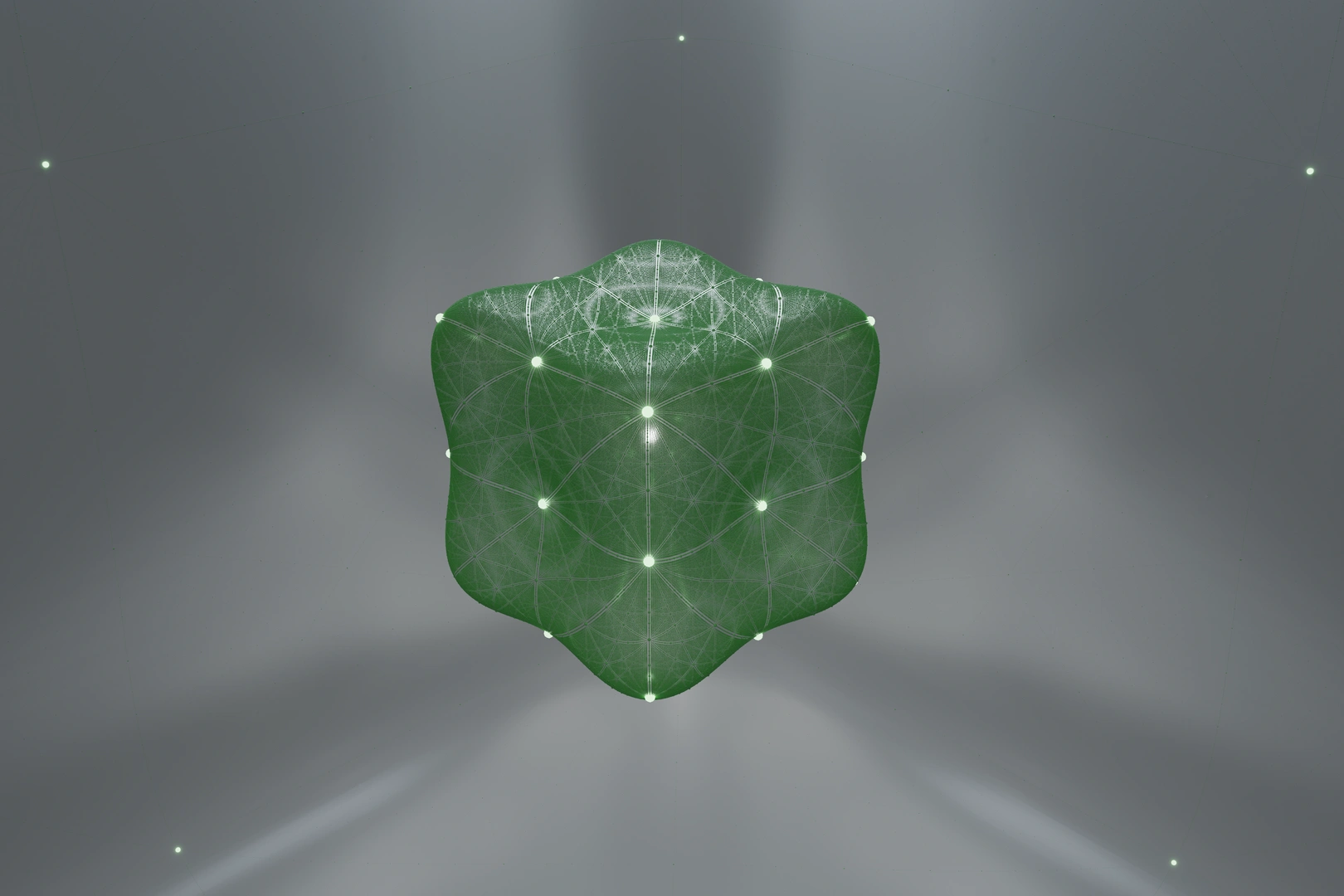
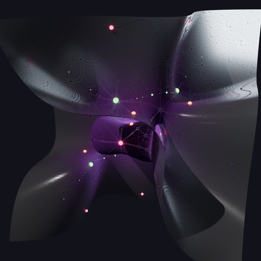
Below is a selection of ray-traced renders created in Blender, highlighting clouds of special points on selected surfaces as small spheres. Usually, points of greatest complexity (except when G = C_1) are rendered as solid objects, while lower-complexity points emit light in order to draw the eye. Points are sized inversely to the (fourth root of) multiplicative Weil height (in terms of the Mahler measure of the primitive, irreducible minimal polynomial).
Footnotes
We can also see some non-dense sets of points—notice how some colors only occur along specific curves!↩︎